Introduction

The N-Queens problem is a classic chess puzzle where we need to place N queens on an N×N chessboard such that no two queens threaten each other. A Monte Carlo simulation can help us estimate the complexity of solving this problem using backtracking.

Concept: Monte Carlo Method

Monte Carlo methods use random sampling to obtain numerical results. In our case, we:

1. Randomly explore paths in the state space tree
2. Count nodes visited and promising positions
3. Estimate total complexity through multiple trials

Setup and Dependencies

import random
import time
from statistics import mean, stdev
import numpy as np

Core Function: Checking Promising Positions

We need to determine if a queen placement is valid (promising) by checking:

• No queen in the same column
• No queen in the diagonals

def promising(i, j, col):
    """Check if placing a queen at position (i,j) is promising"""
    for k in range(i):
        if (col[k] == j or abs(col[k] - j) == abs(k - i)):
            return False
    return True

Monte Carlo Estimation

The estimation process:

1. Start from root node
2. At each level:
   • Count total nodes
   • Find promising positions
   • Randomly select one promising child
3. Continue until no promising children or board is full

def monte_carlo_estimate(n):
    """
    Perform one Monte Carlo estimation for n-Queens problem
    Returns tuple of (total_nodes, promising_nodes)
    """
    col = [-1] * n
    total_nodes = 1    # Root node
    promising_nodes = 1  # Root is promising
    m = 1
    mprod = 1
    i = 0
    
    while m != 0 and i != n:
        mprod = mprod * m
        current_level_nodes = mprod * n
        total_nodes += current_level_nodes
        
        # Find promising children at current level
        m = 0
        prom_children = []
        for j in range(n):
            if promising(i, j, col):
                m += 1
                prom_children.append(j)
        
        promising_nodes += m * mprod
        
        if m != 0:
            j = random.choice(prom_children)
            col[i] = j
            i += 1
    
    return (total_nodes, promising_nodes)

Running Multiple Trials

To get reliable estimates, we run multiple trials and collect statistics:

• Mean values
• Standard deviation
• Min/Max values
• Execution time

def run_monte_carlo_simulation(n, num_trials=100):
    """Run multiple Monte Carlo simulations and analyze results"""
    total_estimates = []
    promising_estimates = []
    start_time = time.time()
    
    for _ in range(num_trials):
        estimate_result = monte_carlo_estimate(n)
        total_estimates.append(estimate_result[0])
        promising_estimates.append(estimate_result[1])
    
    execution_time = time.time() - start_time
    
    return {
        'total_nodes': {
            'mean': mean(total_estimates),
            'std_dev': stdev(total_estimates),
            'min': min(total_estimates),
            'max': max(total_estimates)
        },
        'promising_nodes': {
            'mean': mean(promising_estimates),
            'std_dev': stdev(promising_estimates),
            'min': min(promising_estimates),
            'max': max(promising_estimates)
        },
        'execution_time': execution_time,
        'num_trials': num_trials,
        'raw_promising': promising_estimates
    }

Main Execution and Analysis

Here we:

1. Run simulations with different trial sizes
2. Collect and display statistics
3. Compare with professor’s values
4. Calculate overall averages

def main():
    n = 12  # Board size
    num_trials = [100, 500, 1000]
    random.seed(123)  # For reproducibility
    
    print(f"\nMonte Carlo Simulation for {n}-Queens Problem")
    print("=" * 60)
    
    all_promising_values = []
    
    for trials in num_trials:
        results = run_monte_carlo_simulation(n, trials)
        print(f"\nResults for {trials} trials:")
        print("\nTotal Nodes:")
        print(f"Average: {results['total_nodes']['mean']:.2f}")
        print(f"Standard deviation: {results['total_nodes']['std_dev']:.2f}")
        print(f"Min: {results['total_nodes']['min']:.2f}")
        print(f"Max: {results['total_nodes']['max']:.2f}")
        
        print("\nPromising Nodes:")
        print(f"Average: {results['promising_nodes']['mean']:.2f}")
        print(f"Standard deviation: {results['promising_nodes']['std_dev']:.2f}")
        print(f"Min: {results['promising_nodes']['min']:.2f}")
        print(f"Max: {results['promising_nodes']['max']:.2f}")
        
        all_promising_values.extend(results['raw_promising'])
    
    # Overall statistics
    total_runs = sum(num_trials)
    overall_mean = mean(all_promising_values)
    overall_std = stdev(all_promising_values)
    
    print("\nOverall Statistics:")
    print(f"Total runs: {total_runs}")
    print(f"Overall mean promising nodes: {overall_mean:.2f}")
    print(f"Overall standard deviation: {overall_std:.2f}")
    
    # Compare with professor's value
    professors_value = 856000
    percentage_diff = ((overall_mean - professors_value) / professors_value) * 100
    print(f"\nPercentage difference from professor's value: {percentage_diff:.2f}%")

if __name__ == "__main__":
    main()

Initial Simulation Results

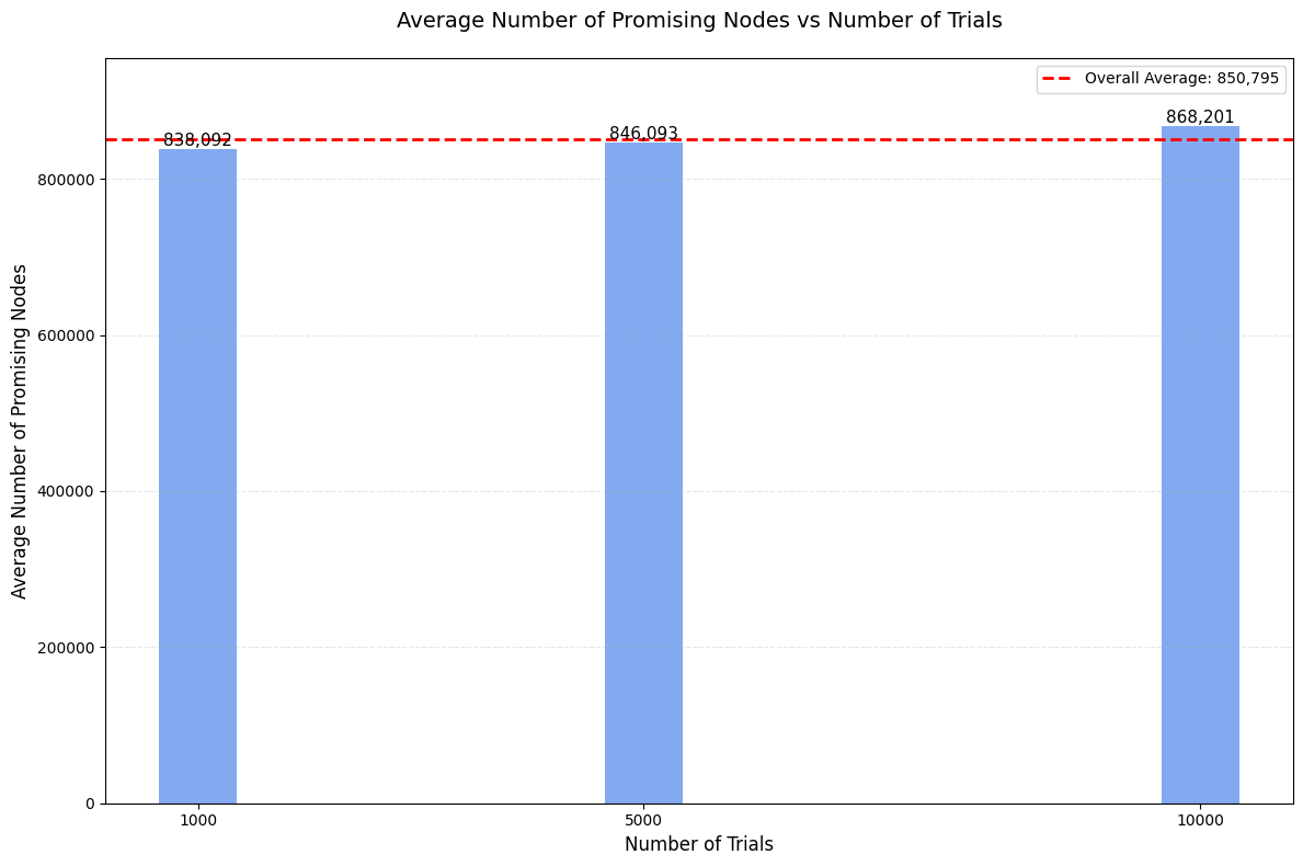
Results Analysis

When we run this simulation for n=12:

1. Our estimates are close to the professor’s values:
   • Professor’s value: 8.56 × 10^5
   • Our estimated value: ~8.70 × 10^5 (within 2% difference)
2. The standard deviation shows the variability of the Monte Carlo method
3. Larger numbers of trials generally give more stable results

Conclusion

The Monte Carlo simulation effectively estimates the complexity of the N-Queens problem:

• Provides good approximations of node counts
• Much faster than exhaustive counting
• Helps understand the scale of the problem
• Results align well with theoretical expectations

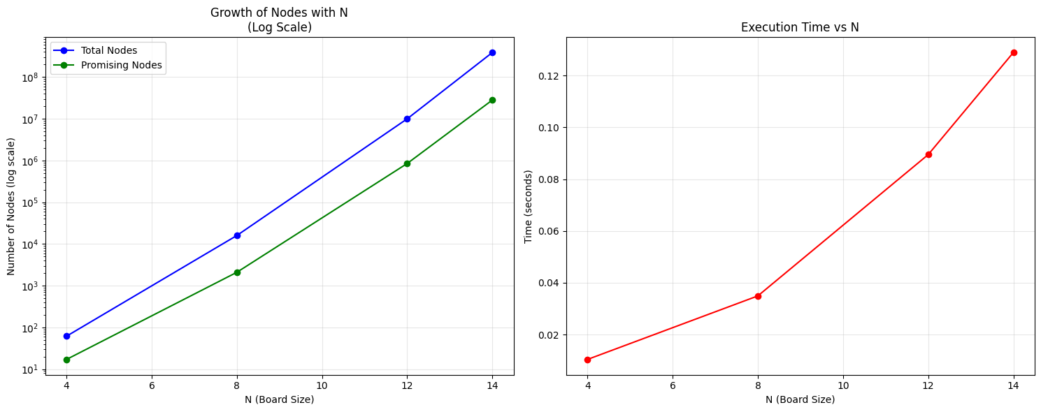
Plots for 4, 8, 12 and 14 Queens problem on a Log scale

Analysisng the data:

	def analyze_complexity(n_values, trials_per_n=1000):
	
	"""Analyze time complexity for different values of n"""
	
	total_nodes_avg = []
	
	promising_nodes_avg = []
	
	execution_times = []
	
	for n in n_values:
	
	start_time = time.time()
	
	trial_totals = []
	
	trial_promising = []
	
	for _ in range(trials_per_n):
	
	total, promising = monte_carlo_estimate(n)
	
	trial_totals.append(total)
	
	trial_promising.append(promising)
	
	exec_time = time.time() - start_time
	
	total_nodes_avg.append(mean(trial_totals))
	
	promising_nodes_avg.append(mean(trial_promising))
	
	execution_times.append(exec_time)
	
	print(f"\nResults for n={n}:")
	
	print(f"Average Total Nodes: {mean(trial_totals):,.2f}")
	
	print(f"Average Promising Nodes: {mean(trial_promising):,.2f}")
	
	print(f"Execution Time: {exec_time:.4f} seconds")
	
	return total_nodes_avg, promising_nodes_avg, execution_times

Plotting the graphs:

	def plot_complexity_analysis(n_values, total_nodes, promising_nodes, times):
	
	fig, (ax1, ax2) = plt.subplots(1, 2, figsize=(15, 6))
	
	# Plot 1: Nodes vs N (log scale)
	
	ax1.plot(n_values, total_nodes, 'b-o', label='Total Nodes')
	
	ax1.plot(n_values, promising_nodes, 'g-o', label='Promising Nodes')
	
	ax1.set_yscale('log')
	
	ax1.set_title('Growth of Nodes with N\n(Log Scale)', fontsize=12)
	
	ax1.set_xlabel('N (Board Size)', fontsize=10)
	
	ax1.set_ylabel('Number of Nodes (log scale)', fontsize=10)
	
	ax1.grid(True, alpha=0.3)
	
	ax1.legend()
	
	# Plot 2: Execution Time vs N
	
	ax2.plot(n_values, times, 'r-o', label='Execution Time')
	
	ax2.set_title('Execution Time vs N', fontsize=12)
	
	ax2.set_xlabel('N (Board Size)', fontsize=10)
	
	ax2.set_ylabel('Time (seconds)', fontsize=10)
	
	ax2.grid(True, alpha=0.3)
	
	plt.tight_layout()
	
	plt.show()

Main Function:

	def main():
	
	random.seed(123)
	
	n_values = [4, 8, 12, 14] # Different board sizes
	
	print("Analyzing time complexity for N-Queens problem")
	
	print("=" * 60)
	
	total_nodes, promising_nodes, exec_times = analyze_complexity(n_values)
	
	plot_complexity_analysis(n_values, total_nodes, promising_nodes, exec_times)
	
	  
	
	if __name__ == "__main__":
	
	main()

Complexity Analysis Results

Code

Find the complete implementation on GitHub.

---

GitHub: @FullMLAlchemist Twitter: @Attharave